CFD simulation of drag: advanced computation for aerodynamics

What is drag?

Drag is a resistance force that opposes the movement of an object as it travels through a fluid, such as air or water.

It is generated by the interaction between the object and the fluid, and manifests itself as fluid friction and pressure forces. Drag is generally expressed in Newtons (N) and is often quantified using a quantity called the drag coefficient.

The use of the drag coefficient goes back centuries, with the first observations and efforts to understand resistance forces in an aerodynamic context. However, it was in the 19th century that scientists, such as George Gabriel Stokes, began to formalise the concept and develop mathematical theories to quantify drag. Since then, drag research has played an essential role in the development of aviation, the automobile, building design and many sporting activities.

In short, drag is a resistance force encountered when an object moves through a fluid; the drag coefficient quantifies it. Understanding and mastering drag is essential to optimise the performance, efficiency and safety of moving objects.

The importance of the drag coefficient

The drag coefficient is a measure that quantifies the resistance of air or a fluid to the movement of an object. It plays a key role in aviation, the automobile, in gliding sports or even in building architecture. Understanding and mastering this resistance force is crucial to optimise the performance and efficiency of many applications.

In aviation, reducing drag is a major concern: by minimising this resistance, engineers can increase the speed and energy efficiency of aircraft, reduce fuel consumption and improve their range. Advances have also been made in improving the lift of aircraft (detailed later), leading to significant progress in wing design.

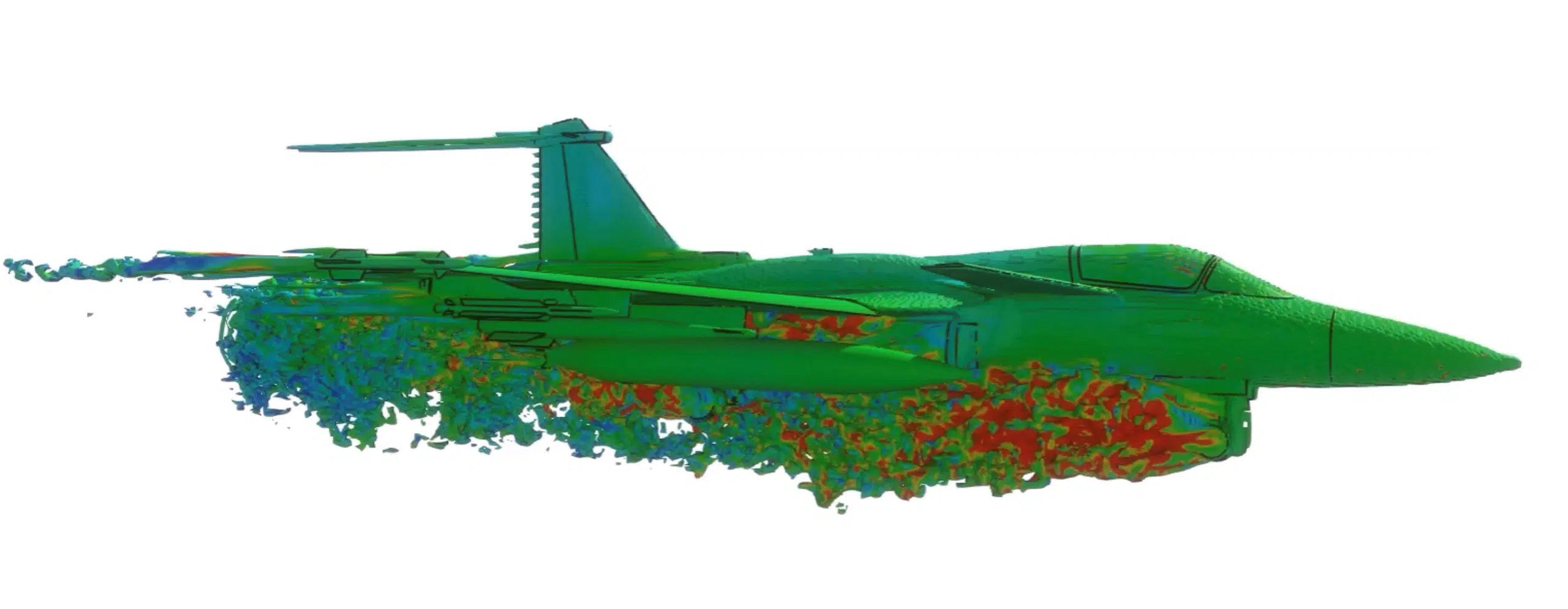
The automotive industry also seeks to minimise this drag to reduce the energy consumption of cars and improve their range — an issue all the more topical with the emergence of electric vehicles. Motor sports (such as Formula 1), for their part, seek to maximise aerodynamics to improve roadholding, stability and performance.

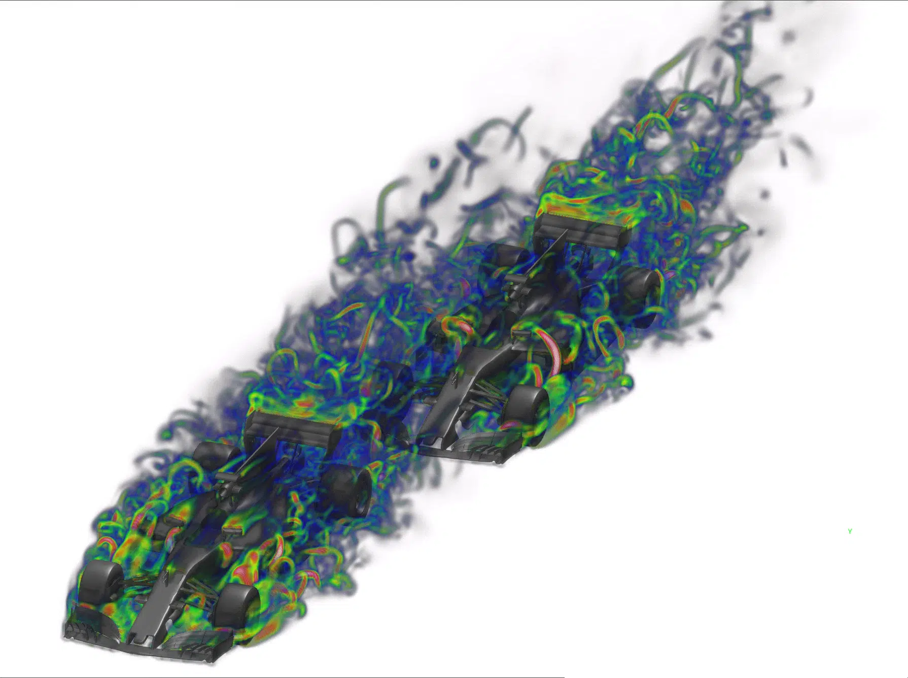
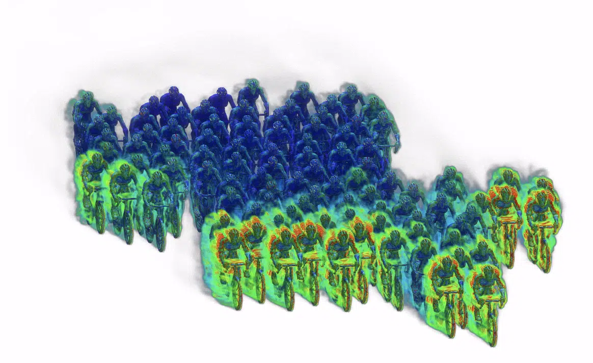
Likewise, in gliding sports (alpine skiing, snowboarding) or cycling, reducing drag makes it possible to reach higher speeds by minimising resistance forces and optimising penetration through the air. This leads to advances in the design of cycling helmets and other sporting equipment.

Building architecture is also influenced by the principles of drag: by designing aerodynamic structures, architects reduce the forces exerted by high winds and improve the safety and stability of constructions (bridges, for example).

The drag coefficient is therefore a crucial measure in all fields that involve an interaction between an object and a fluid.

Computing the drag coefficient

Definition

The drag force, denoted D (for Drag), is given by the following formula:

This force therefore depends on the characteristics of the fluid (density), the object (shape and roughness) and the relative speed between the object and the fluid. The drag coefficient C_x is obtained by relating the drag force to the dynamic pressure and the reference area:

It should be noted that the drag coefficient is not a constant quantity: it depends on the properties of the flowing fluid, the shape of the object and the surface roughness. More rigorously, it can be shown that the coefficient C_D depends on the Reynolds number.

Note — the lift coefficient (or downforce coefficient in some cases) is defined in the same way:

Drag coefficient and Reynolds number

The Reynolds number (Re) is a dimensionless quantity that characterises the flow regime of a fluid. It is calculated by dividing the product of the speed, the characteristic length and the density of the fluid by its viscosity:

The Reynolds number makes it possible to determine whether the flow is laminar (low Re) or turbulent (high Re). A laminar flow corresponds to fluid particles moving in regular, ordered layers; a turbulent flow is characterised by chaotic and irregular movements.

It can be shown that the drag coefficient depends on the Reynolds number. For a smooth sphere (red curve below), C_x first decreases as the Reynolds number increases, then stabilises around a constant value. There is a narrow range at high Reynolds for which C_x drops then rises again: this phenomenon, called the drag crisis, marks the transition from a laminar flow to turbulence — linked to a later boundary-layer separation on the surface.

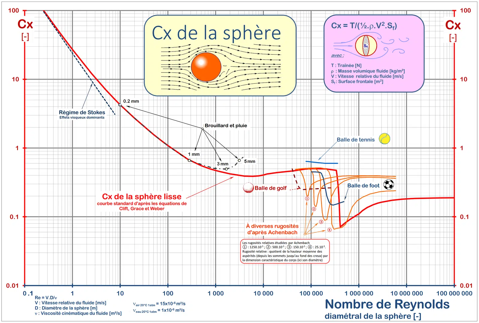
Take the example of the golf ball: the surface dimples promote the transition to turbulence and allow a reattachment of the boundary layer. With a Reynolds number between 10⁴ and 10⁵, the ball lies in the drag-crisis region, which allows it to travel greater distances.

Influence of a body's shape on drag

The shape of a body has a major influence on the drag force. Objects with a streamlined or aerodynamic shape (aircraft, racing cars) generally have lower drag coefficients, thanks to a reduced interaction area with the air and a smoother, more laminar flow.

Conversely, objects with a flat or angular shape (trucks, buildings) have higher coefficients: these shapes create more turbulence and air vortices, increasing the resistance to flow and the drag.

Vehicle aerodynamics

The concept of the boundary layer

The boundary layer is a thin region near the surface of an object where the effects of the fluid viscosity become significant: the fluid speed near the surface is slowed by friction. It plays a crucial role in the transition between laminar and turbulent flows, and in the formation of the wake behind moving objects.

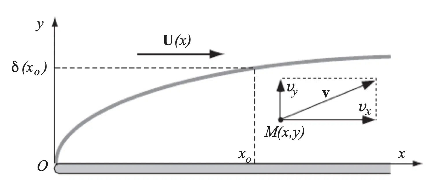
The concept of the boundary layer, developed by Ludwig Prandtl in 1905, must be adjusted to suit practical situations, in particular in the presence of turbulent flows upstream of a body: these conditions modify the velocity profiles, with the appearance of a turbulent boundary layer.

When solid bodies are poorly streamlined, this can lead to boundary-layer separation, generating a turbulent wake downstream. The flow then no longer behaves like an ideal fluid, leading to a notable increase in energy dissipation and drag force.

Aircraft wing — boundary-layer control

The important aerodynamic force for an aircraft wing is the lift force. It is generated by the Magnus effect thanks to the circulation of velocity around the wing. To keep the aircraft in flight, the lift force (F_L) must offset its weight. This force grows proportionally to the square of the speed and linearly with the angle of attack (α) when the latter is small:

The more the angle α increases, the more the lift increases — this is the desired effect. However, when α exceeds a critical value α_c, the phenomenon of stall occurs: the lift drops sharply and the formula is no longer valid. It is therefore to be avoided, particularly in civil aviation.

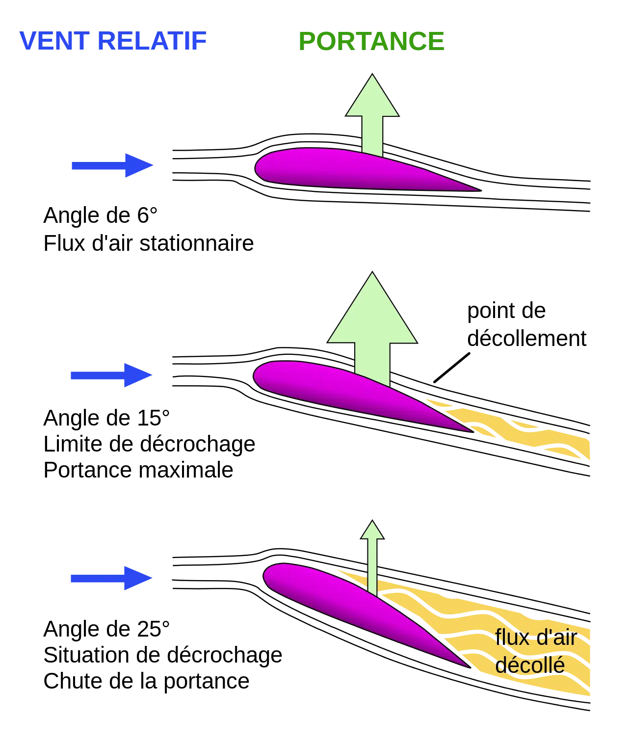
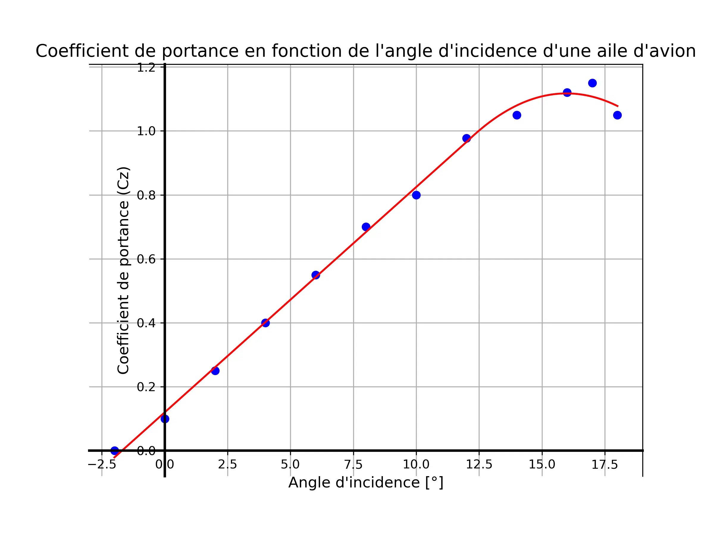
Two common approaches to improve wing performance: increasing the critical angle of attack using leading-edge slats, and increasing the lift coefficient for a given angle using trailing-edge flaps.

The leading-edge slats increase the critical angle of attack by re-energising the upper-surface boundary layer through the injection of tangential air from the lower surface, which reduces the effect of the adverse pressure gradient at high angles.

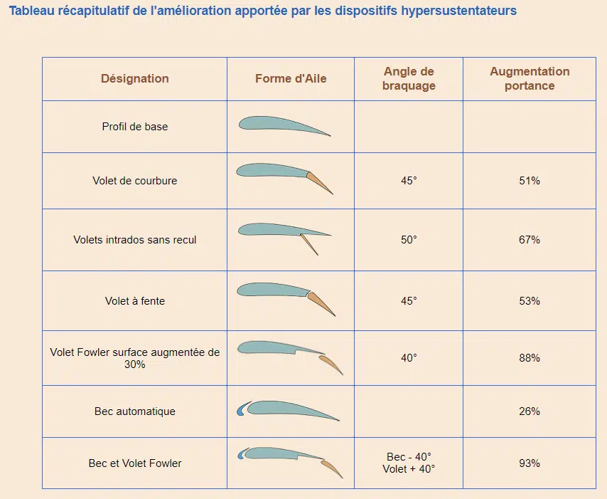
The trailing-edge flaps increase the circulation around the wing profile, raising the lift for a given angle of attack. On large aircraft, these flaps can be used in series to increase lift at take-off and landing: they re-energise the upper-surface boundary layer and induce a strong downward deflection of the flow velocity.

The case of land vehicles

Stakes — for land vehicles, minimising the drag force is crucial to improve energy efficiency. This force is mainly generated by the pressure difference between the front and the rear of the vehicle. Unlike aircraft, where friction with the air dominates, pressure here plays a predominant role.

An important feature of cars is that the lift force must be directed downwards to maintain good tyre grip. This contributes to better roadholding; but excessive downforce can lead to premature tyre wear and excessive friction. Finding the right balance between reducing drag and maintaining sufficient downforce is a challenge for automotive engineers.

Drag reduction — the effort focuses in particular on more aerodynamic body shapes. Over the years, manufacturers have reduced the drag coefficient (C_x), down from more than 0.5 for older cars to less than 0.3 for modern vehicles, improving energy efficiency and reducing consumption.

However, drag reduction must be balanced against other requirements (interior space, visibility), which calls for compromises. A large part of the drag is generated at the rear of the vehicle, where boundary-layer separations and vortex formation affect the resistance. Engineers use standard models such as the Ahmed body to study the impact of parameters such as the rear-window angle.

Studies reveal that drag varies non-monotonically with the slant angle: at low angles, the contribution of the transverse recirculation can be reduced while the effect of the axial vortices is amplified. This underlines the complexity of vehicle aerodynamics. Finally, maintaining sufficient negative lift guarantees good roadholding at high speed. For Formula 1 cars, which run at around 250 km/h, systems such as wings improve downforce — at the cost of increased drag.

Active or passive control of drag or lift

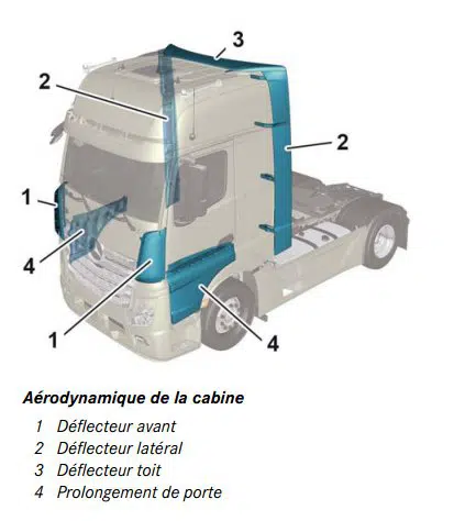
Aerodynamic improvements — adding roof deflectors to trucks, modifying the shape of mirrors — can reduce drag passively, without any energy input. In active control, the action is adjusted in real time according to the flow conditions, either manually by the driver (open loop), or automatically by a computer (closed loop).

For example, to prevent boundary-layer separation, one can suck in or inject air near the wall to maintain a stable flow — although this requires additional power and is rarely used in practice. Closed-loop reactive control, still in the research phase, involves devices such as motorised vortex generators, with potential applications notably in aeronautics.

Computing the drag coefficient in CFD simulation

Advantages of CFD simulation

The use of computational fluid dynamics (CFD) offers several advantages over traditional wind-tunnel testing. First, CFD makes it possible to carry out virtual simulations, avoiding the costs and delays associated with building and operating physical wind tunnels (specialised facilities, costly models, precise measurement equipment).

Then, CFD offers greater flexibility in the design and study parameters: it is easier to modify the geometry of the object, the flow conditions or the fluid properties. This makes it possible to explore a larger number of scenarios and to optimise the design more efficiently.

In addition, CFD offers better visualisation and more detailed analysis: streamlines, turbulence zones, pressure gradients… all information that helps to better understand the aerodynamic phenomena and identify areas for improvement.

Finally, CFD makes it possible to explore a wider range of flow conditions: extreme conditions, high speeds, different temperatures… offering greater flexibility to test and validate performance under real conditions — which EOLIOS is able to carry out.

Determining the aerodynamic coefficients

To determine the drag coefficient (and the lift coefficient), whether in CFD simulation or by experimental method, one must understand the pressure distribution over the surface of the body. The viscous shear forces must also be taken into account over the entire surface.

By integrating the pressure distribution over the surface of the object, one can derive the drag force and the drag coefficient. Thanks to CFD software, the value of the aerodynamic coefficients can be predicted directly after the simulation.

Determining the aerodynamic coefficients is a crucial step in the design and optimisation of any object subject to aerodynamic forces. This information improves performance in terms of drag, lift and stability, and is essential in aeronautics, the automobile or sport.

CFD simulation of a Formula 1 car

Context

Aerodynamics plays a crucial role in the performance of Formula 1 cars, where every millisecond counts. A well-designed car can generate high levels of downforce, improving tyre grip and allowing higher cornering speeds; reducing drag makes it possible to reach higher top speeds on the straights.

In this context, CFD simulation has become an indispensable tool for Formula 1 teams. It makes it possible to numerically model the behaviour of the airflow around the car (speed, pressure, turbulence) and provides crucial information on how aerodynamic configurations affect performance — in particular the values of the aerodynamic coefficients and forces.

In this context, EOLIOS carried out simulations on a Formula 1 car to determine these aerodynamic coefficients and highlight the phenomena responsible for the various forces.

Velocity field

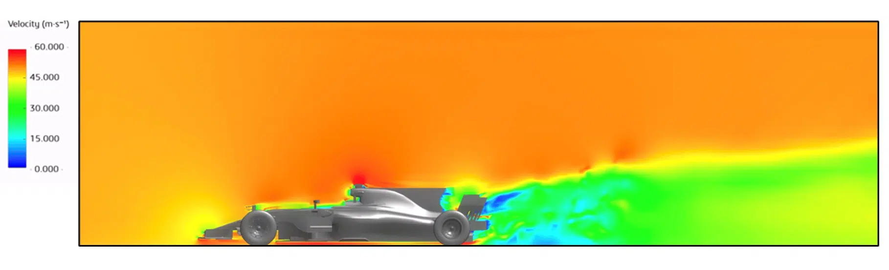
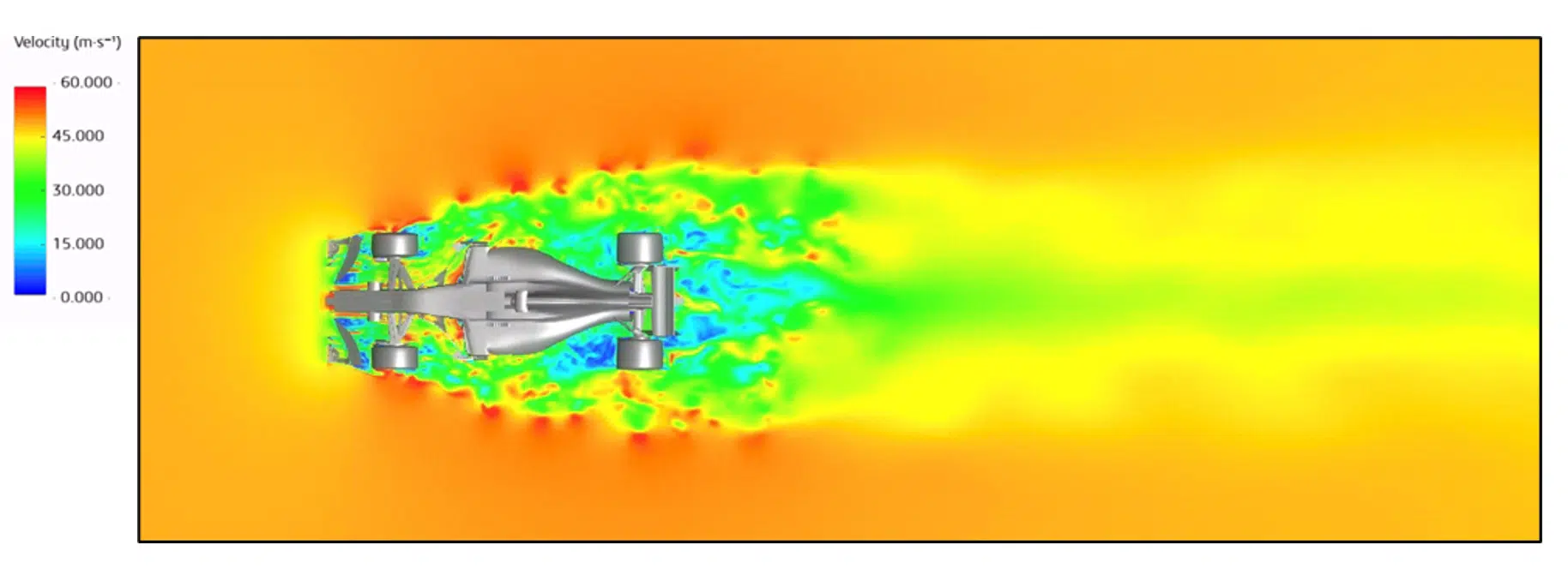
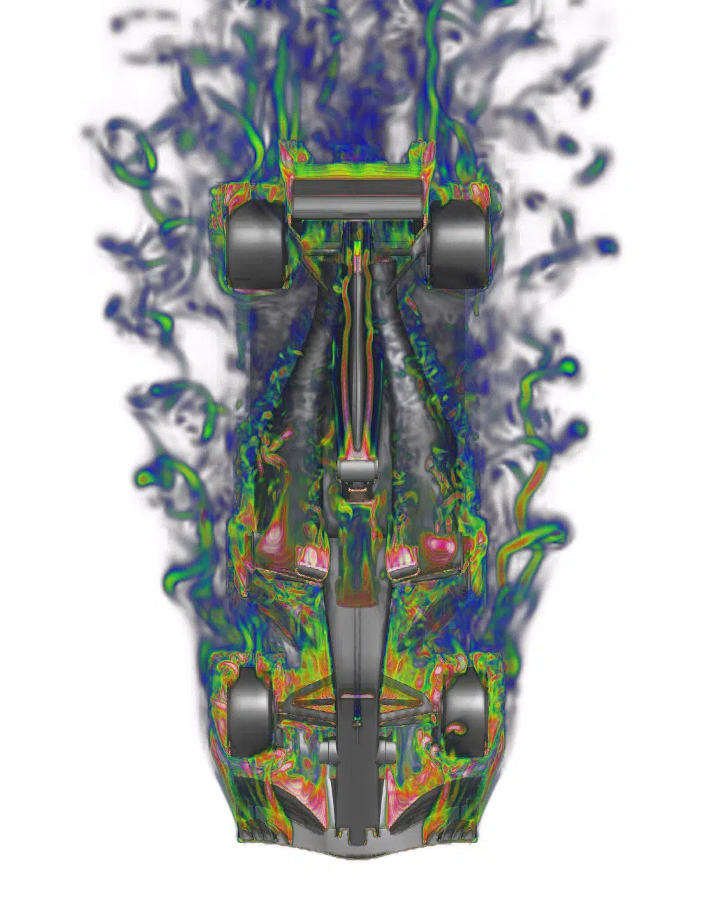
The main observation is that the presence of the car significantly disturbs the surrounding velocity field, particularly at the rear where the flow is “very disturbed and disordered” — characteristics typical of a turbulent flow.

Turbulent flow is distinguished by its irregularity and complexity, resulting from the formation of vortices, pressure fluctuations and chaotic movements. It can be generated by the separation of the boundary layer around the bodywork and the interactions with the surrounding air. These characteristics increase the aerodynamic drag, reduce energy efficiency and heighten instability at high speed: understanding them is essential to optimise the design.

Drag force

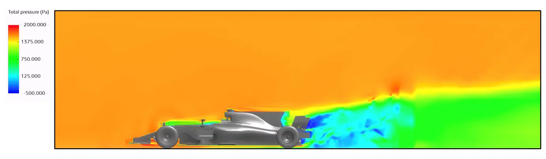
Behind the car, a low-pressure zone can be observed which is largely responsible for the drag. The swirling flow behind the car is detrimental to aerodynamics: the air struggles to flow around the object, creating an overpressure at the front and then a low pressure at the rear.

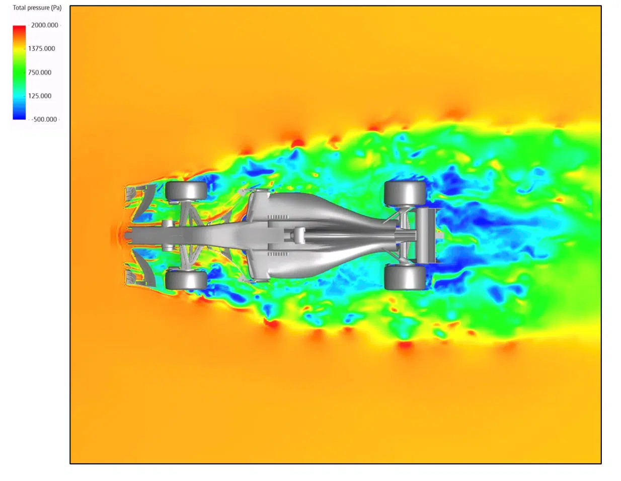
In competition, on the straights, drivers take advantage of this low pressure behind the vehicle ahead of them to overtake: the following car no longer has to “cut through” the air, and the pressure difference between the front and the rear — and therefore the drag — are reduced. It is said to benefit from the “slipstream”.

The CFD simulation software makes it possible to determine the values of the forces and aerodynamic coefficients. In our simulations, the drag coefficient is estimated at around 0.92 (a standard value for an F1 car) and the drag force is F = 1900 N. The theoretical calculation with an area S = 1.5 m² gives F_d = 2070 N, close to the simulated value (the area S used for this order of magnitude being approximate).

Vorticity

Vorticity measures the rotation of a fluid around a local axis. When an object passes through a fluid, it disturbs its flow and creates vortices where the speed and direction change; these vortices generate vorticity, indicating the intensity and location of the rotations.

On the vorticity planes, one observes how the presence of the car influences the flow: the zones of high vorticity correspond to the places where the vortices are most intense, often downstream and on the sides of the car.

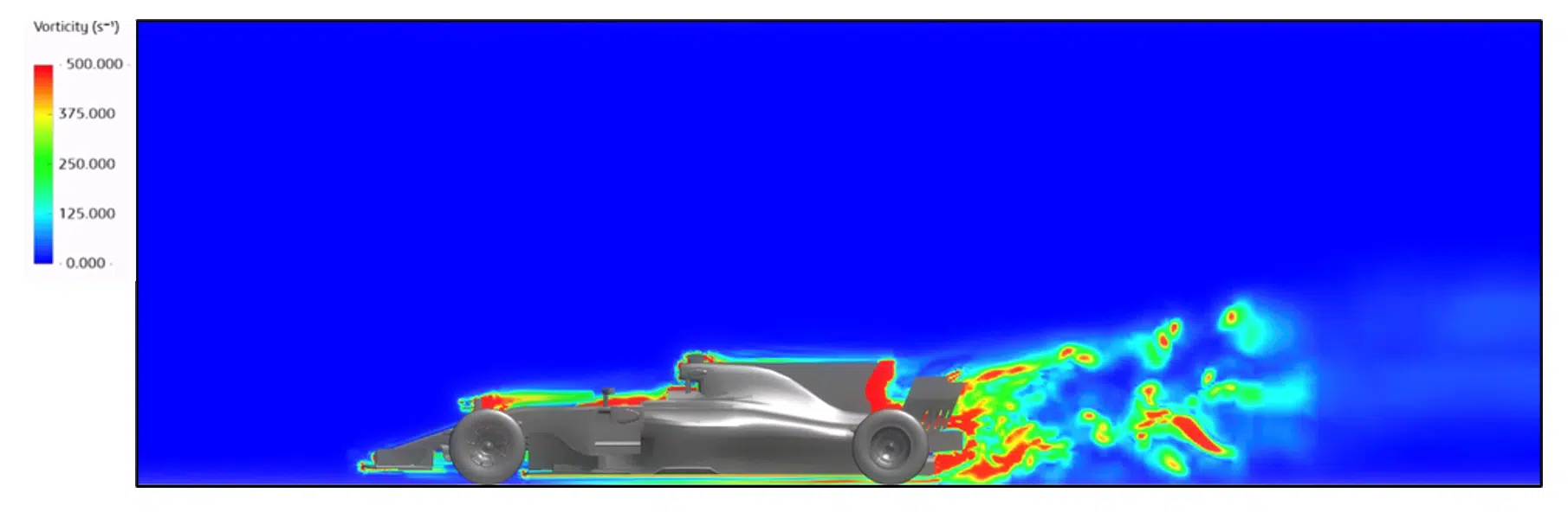
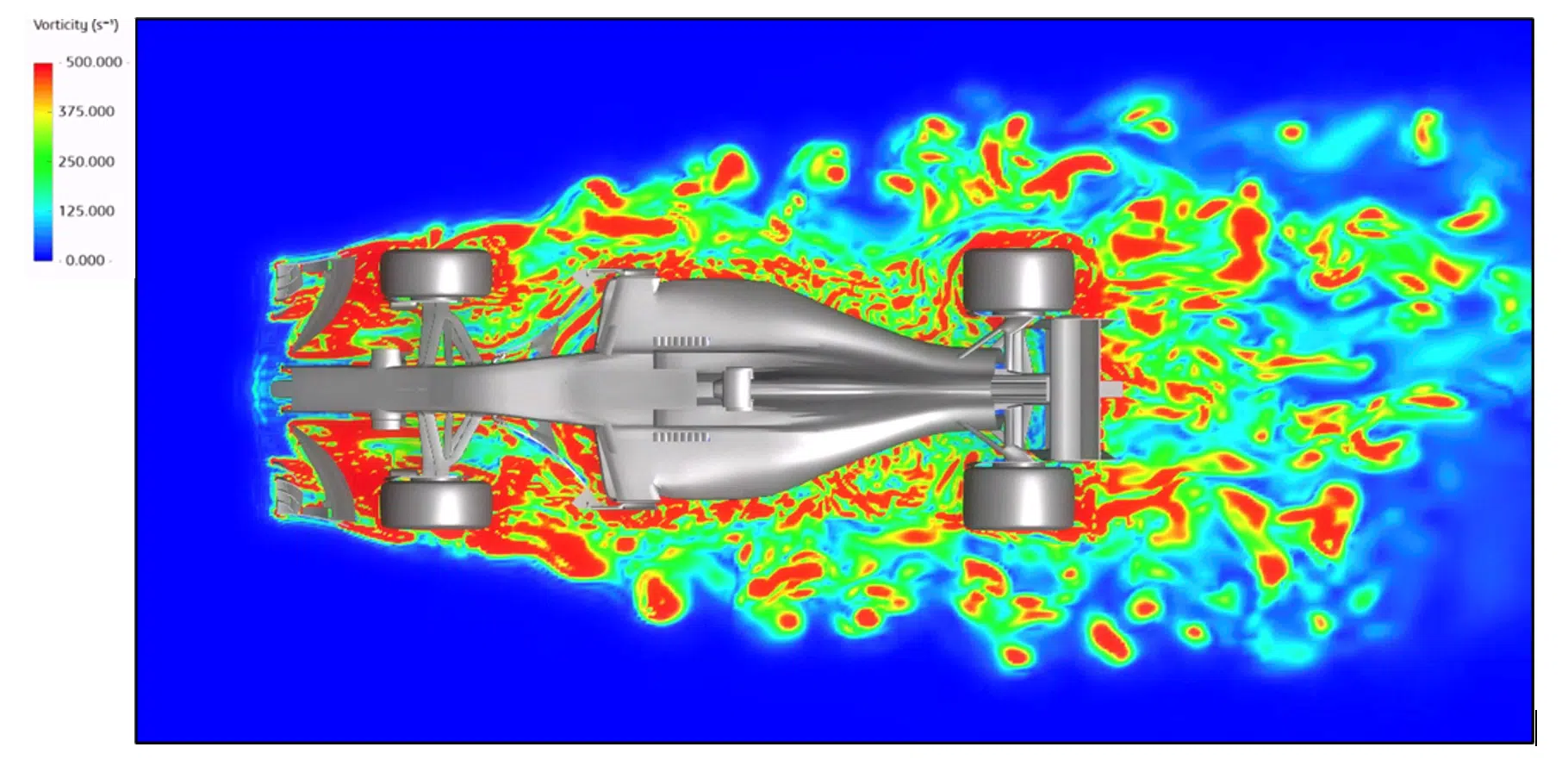
The visual analysis carried out with these simulations makes it possible to better understand the interaction between the moving car and the surrounding fluid — crucial for the aerodynamics of Formula 1 cars.

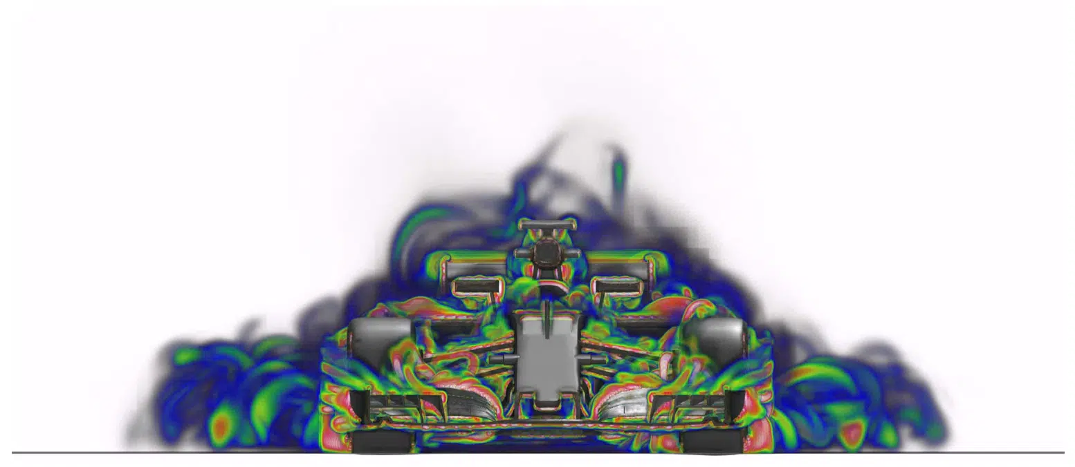
The “slipstream” effect: an F1 car in the act of overtaking

Another simulation aims to estimate the drag force of a racing car when it experiences the slipstream of the vehicle ahead of it, just before overtaking. The configuration examined is shown below.

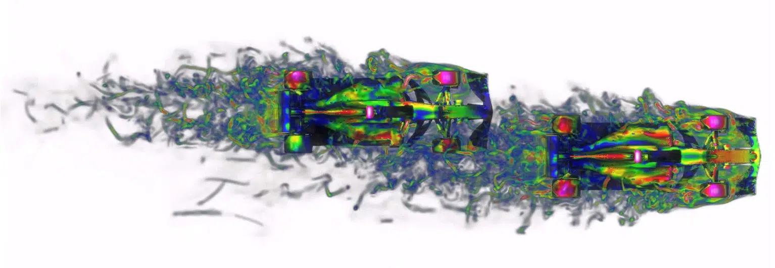
When one Formula 1 car overtakes another, the aerodynamic forces acting on each car are greatly influenced by their relative position. The overtaking car benefits from a significant reduction in air resistance thanks to the slipstream effect generated by the car ahead of it: it gains speed while requiring less power.

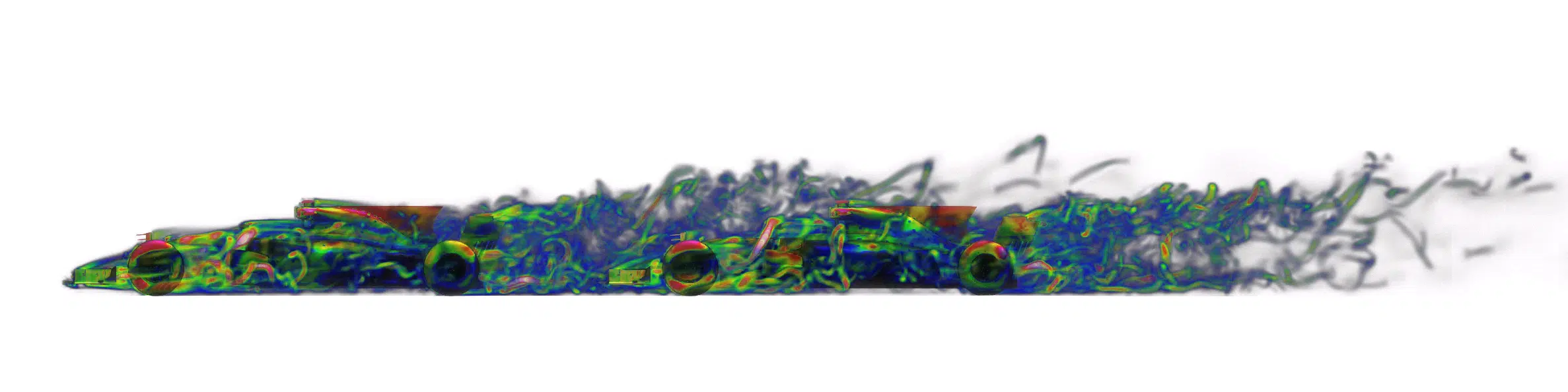
Moreover, the overtaken car experiences an increase in its drag coefficient because of the disturbance to the airflow caused by the proximity of the car behind it. These phenomena show how closely racing dynamics are tied to aerodynamic interactions, and underline the importance of positioning and drag management in the overtaking strategy.

Optimising aerodynamics with CFD

Aerodynamic forces, in particular drag, play a crucial role in many fields — from aeronautics to the automobile, by way of sports and buildings. Understanding and minimising these forces improves the efficiency, safety and durability of vehicles and structures. CFD simulation is emerging as an essential tool, far more accessible and economical than wind-tunnel testing.

It allows a detailed analysis of the aerodynamic phenomena, paving the way for higher-performing designs and faster innovation across various sectors.