Why pressure loss decides an entire network
As soon as a fluid — air, water, smoke — flows through a duct, a conduit or pipework, it rubs against the walls and meets changes of direction. With every metre travelled, it loses energy: this is pressure loss.
Underestimating this loss means choosing a fan or pump that is too weak and never reaching the target flow rate. Overestimating it means oversizing the installation and wasting energy continuously. Calculating it well means sizing it right.
What is a pressure loss?
The pressure loss (written ΔP) is the pressure drop experienced by a moving fluid, caused by the viscous dissipation of its energy through friction and turbulence. It is expressed in pascals (Pa) and grows, for the most part, with the square of the flow speed.
Two families of losses are distinguished, which add up across the whole network:
Friction losses (linear)
- Caused by friction along the walls of a straight duct.
- Proportional to length and inversely to diameter.
Local losses (fittings)
- Caused by fittings: bends, tees, valves, expansions, grilles.
- Concentrated at a point, but often dominant.
The flow regime: laminar or turbulent?
Before any calculation, the nature of the flow must be known. The Reynolds number compares inertial forces with viscous forces and determines whether the fluid flows in parallel streamlines (laminar) or chaotically (turbulent).
In almost all air and water networks in buildings and industry, the flow is turbulent: it is this regime that governs the calculation methods below.
Friction losses: the Darcy-Weisbach equation
Over a straight length of duct, the pressure loss is calculated using the universal Darcy-Weisbach relation:
The coefficient λ depends on the Reynolds number and the relative roughness of the wall. It is classically read on the Moody diagram or computed with the Colebrook equation. The practical lesson: since ΔP varies as V², doubling the speed multiplies the loss by four — hence the value of generously sized ducts.
Local losses: the K coefficient
Each fitting in the network — bend, tee, reducer, damper, grille — causes a local loss, modelled by a local-loss coefficient K:
On a compact network, these local losses often dominate the linear losses. Smoothing a sharp bend, streamlining a junction or enlarging a grille can cut the overall loss far more effectively than widening the straight ducts.
Charts stop where geometry becomes real
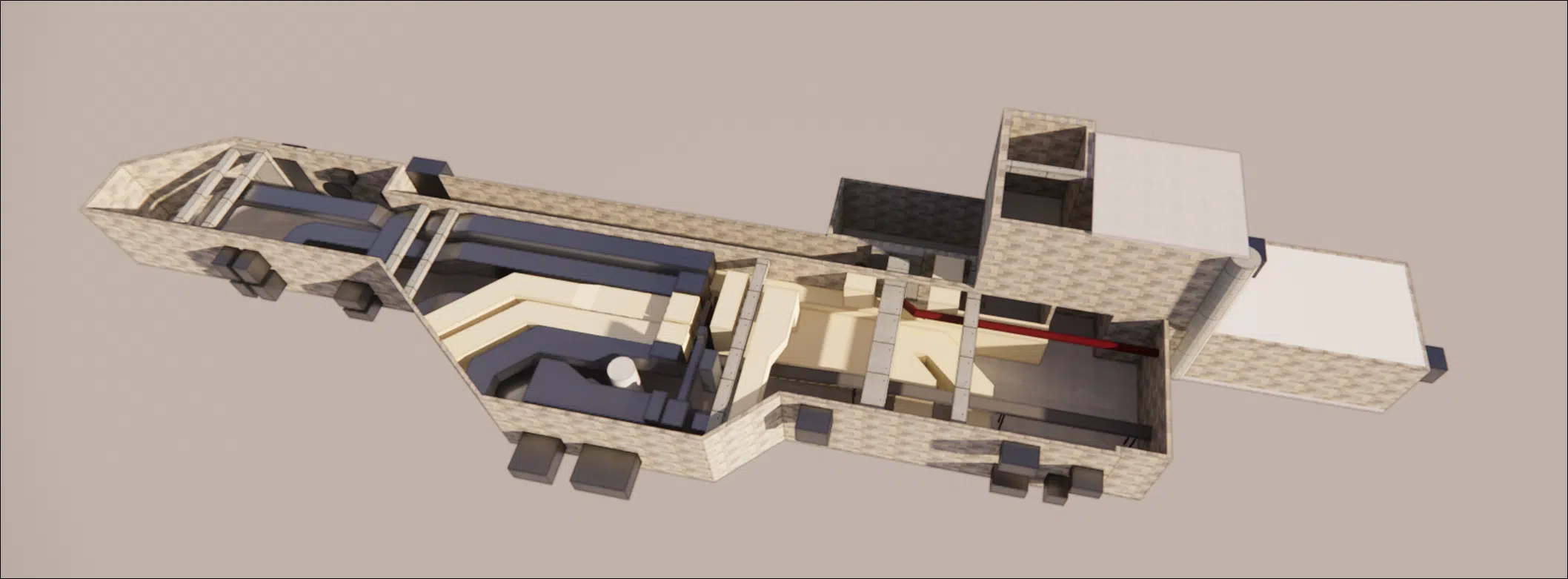
Tabulated K coefficients hold for isolated, ideal fittings. As soon as two bends follow one another, a junction is asymmetric or a hopper is cluttered, the interaction between fittings falls outside the charts: only CFD then gives a reliable value.
Hydraulic resistance & network balancing
At the scale of a complete network, we speak of hydraulic resistance: the overall opposition the installation offers to the passage of the fluid. Crossed with the fan or pump curve, it sets the real operating point (the flow rate and pressure actually obtained).
When several branches share one flow, the challenge becomes balancing: distributing the flow rates correctly between branches so that no zone is over-supplied at the expense of another. A poorly balanced network means badly ventilated spaces and control devices that "eat" energy for nothing.
When CFD simulation takes over from the charts
Formulae and charts are enough for a regular network. But as soon as the geometry becomes complex or constrained — cluttered hoppers, plenums, air intakes, multiple junctions, heat exchangers — CFD simulation becomes the reference tool.
It computes the real pressure loss of the exact geometry, visualises the recirculation and separation zones that dissipate energy, and lets you test routing variants before manufacturing. The result is the tightest possible sizing, without oversizing "to be safe".
Case study: pressure losses — the CNIT networkOur engineers quantify your pressure losses and optimise the routing through CFD simulation. Let's talk.